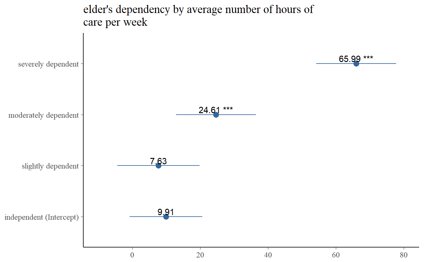
Plot One-Way-Anova tables

Plot One-Way-Anova table sum of squares (SS) of each factor level (group) against the dependent variable. The SS of the factor variable against the dependent variable (variance within and between groups) is printed to the model summary.

sjp.aov1(var.dep, var.grp, meansums = FALSE, title = NULL,
  axis.labels = NULL, rev.order = FALSE, string.interc = "(Intercept)",
  axis.title = "", axis.lim = NULL, geom.colors = c("#3366a0", "#aa3333"),
  geom.size = 3, wrap.title = 50, wrap.labels = 25, grid.breaks = NULL,
  show.values = TRUE, digits = 2, y.offset = 0.1, show.p = TRUE,
  show.summary = FALSE, prnt.plot = TRUE)

Arguments

var.dep	Dependent variable. Will be used with following formula: aov(var.dep ~ var.grp)
var.grp	Factor with the cross-classifying variable, where var.dep is grouped into the categories represented by var.grp.
meansums	Logical, if TRUE, the values reported are the true group mean values (see also sjt.grpmean). If FALSE (default), the values are reported in the standard way, i.e. the values indicate the difference of the group mean in relation to the intercept (reference group).
title	character vector, used as plot title. Depending on plot type and function, will be set automatically. If title = "", no title is printed. For effect-plots, may also be a character vector of length > 1, to define titles for each sub-plot or facet.
axis.labels	character vector with labels used as axis labels. Optional argument, since in most cases, axis labels are set automatically.
rev.order	Logical, if TRUE, order of categories (groups) is reversed.
string.interc	Character vector that indicates the reference group (intercept), that is appended to the value label of the grouping variable. Default is "(Intercept)".
axis.title	Character vector of length one or two (depending on the plot function and type), used as title(s) for the x and y axis. If not specified, a default labelling is chosen. To set multiple axis titles (e.g. with type = "eff" for many predictors), axis.title must be a character vector of same length of plots that are printed. In this case, each plot gets an own axis title (applying, for instance, to the y-axis for type = "eff"). Note: Some plot types do not support this argument. In such cases, use the return value and add axis titles manually with labs, e.g.: $plot.list[[1]] + labs(x = ...)
axis.lim	Numeric vector of length 2, defining the range of the plot axis. Depending on plot type, may effect either x- or y-axis, or both. For multiple plot outputs (e.g., from type = "eff" or type = "slope" in sjp.glm), axis.lim may also be a list of vectors of length 2, defining axis limits for each plot (only if non-faceted).
geom.colors	user defined color for geoms. See 'Details' in sjp.grpfrq.
geom.size	size resp. width of the geoms (bar width, line thickness or point size, depending on plot type and function). Note that bar and bin widths mostly need smaller values than dot sizes.
wrap.title	numeric, determines how many chars of the plot title are displayed in one line and when a line break is inserted.
wrap.labels	numeric, determines how many chars of the value, variable or axis labels are displayed in one line and when a line break is inserted.
grid.breaks	numeric; sets the distance between breaks for the axis, i.e. at every grid.breaks'th position a major grid is being printed.
show.values	Logical, whether values should be plotted or not.
digits	Numeric, amount of digits after decimal point when rounding estimates and values.
y.offset	numeric, offset for text labels when their alignment is adjusted to the top/bottom of the geom (see hjust and vjust).
show.p	Logical, adds significance levels to values, or value and variable labels.
show.summary	logical, if TRUE (default), a summary with chi-squared statistics (see chisq.test), Cramer's V or Phi-value etc. is shown. If a cell contains expected values lower than five (or lower than 10 if df is 1), the Fisher's excact test (see fisher.test) is computed instead of chi-squared test. If the table's matrix is larger than 2x2, Fisher's excact test with Monte Carlo simulation is computed.
prnt.plot	logical, if TRUE (default), plots the results as graph. Use FALSE if you don't want to plot any graphs. In either case, the ggplot-object will be returned as value.

Value

(Insisibily) returns the ggplot-object with the complete plot (plot) as well as the data frame that was used for setting up the ggplot-object (df).

See also

sjt.grpmean

Examples

data(efc)
# note: "var.grp" does not need to be a factor.
# coercion to factor is done by the function
sjp.aov1(efc$c12hour, efc$e42dep)